
This topic describes the rules for selecting the access path in OceanBase AI Database.
Currently, the rules for selecting the access path in OceanBase AI Database are classified into pre-rules (forward rules) and skyline pruning rules (reverse rules). Pre-rules directly determine which index is used by a query and are a strong-matching rule system.
Skyline pruning rules compare two indexes. If an index dominates another index in some defined dimensions, the inferior index is pruned. The remaining unpruned indexes are then compared based on cost to select the optimal execution plan.
The optimizer of OceanBase AI Database prioritizes using pre-rules to select indexes. If no matching index is found, skyline pruning rules prune out some less optimal indexes. Finally, the cost model selects the path with the lowest cost from the unpruned indexes.
As shown in the following example, OceanBase AI Database displays the information about a path selection rule in the plan demonstration.
Create table
t1.obclient> CREATE TABLE t1(a INT PRIMARY KEY, b INT, c INT, d INT, e INT, UNIQUE INDEX k1(b), INDEX k2(b,c), INDEX k3(c,d) );View the execution plan with the query condition
b = 1.obclient> EXPLAIN EXTENDED SELECT * FROM t1 WHERE b = 1;The result is as follows:
+--------------------------------------------------------------------------------------------------------------------------------------------------------------+ | Query Plan | +--------------------------------------------------------------------------------------------------------------------------------------------------------------+ | =========================================== | | |ID|OPERATOR |NAME |EST.ROWS|EST.TIME(us)| | | ------------------------------------------- | | |0 |TABLE GET|t1(k1)|1 |10 | | | =========================================== | | Outputs & filters: | | ------------------------------------- | | 0 - output([t1.a(0x7f7c3b2235a0)], [t1.b(0x7f7c3b223320)], [t1.c(0x7f7c3b223730)], [t1.d(0x7f7c3b2238c0)], [t1.e(0x7f7c3b223a50)]), filter(nil), rowset=16 | | access([t1.a(0x7f7c3b2235a0)], [t1.b(0x7f7c3b223320)], [t1.c(0x7f7c3b223730)], [t1.d(0x7f7c3b2238c0)], [t1.e(0x7f7c3b223a50)]), partitions(p0) | | is_index_back=true, is_global_index=false, | | range_key([t1.b(0x7f7c3b223320)], [t1.shadow_pk_0(0x7f7c3b2c8550)]), range[1,NULL ; 1,NULL], | | range_cond([t1.b(0x7f7c3b223320) = 1(0x7f7c3b223080)(0x7f7c3b2231d0)]) | | Used Hint: | | ------------------------------------- | | /*+ | | | | */ | | Qb name trace: | | ------------------------------------- | | stmt_id:0, stmt_type:T_EXPLAIN | | stmt_id:1, SEL$1 | | Outline Data: | | ------------------------------------- | | /*+ | | BEGIN_OUTLINE_DATA | | INDEX(@"SEL$1" "test_db"."t1"@"SEL$1" "k1") | | OPTIMIZER_FEATURES_ENABLE('4.5.0.0') | | END_OUTLINE_DATA | | */ | | Optimization Info: | | ------------------------------------- | | t1: | | table_rows:1 | | physical_range_rows:1 | | logical_range_rows:1 | | index_back_rows:1 | | output_rows:1 | | table_dop:1 | | dop_method:Table DOP | | avaiable_index_name:[k1, k2, k3, t1] | | pruned_index_name:[k2, k3, t1] | | stats info:[version=1970-01-01 08:00:00.000000, is_locked=0, is_expired=0] | | dynamic sampling level:0 | | estimation method:[DEFAULT] | | Plan Type: | | LOCAL | | Parameters: | | :0 => 1 | | Note: | | Degree of Parallelisim is 1 because of table property | +--------------------------------------------------------------------------------------------------------------------------------------------------------------+ 50 rows in setView the execution plan with the query conditions
c < 5and the sortingORDER BY c.obclient> EXPLAIN EXTENDED SELECT * FROM t1 WHERE c < 5 ORDER BY c;The result is as follows:
+--------------------------------------------------------------------------------------------------------------------------------------------------------------+ | Query Plan | +--------------------------------------------------------------------------------------------------------------------------------------------------------------+ | ================================================== | | |ID|OPERATOR |NAME |EST.ROWS|EST.TIME(us)| | | -------------------------------------------------- | | |0 |TABLE RANGE SCAN|t1(k3)|1 |5 | | | ================================================== | | Outputs & filters: | | ------------------------------------- | | 0 - output([t1.a(0x7f7c3b223a60)], [t1.b(0x7f7c3b223bf0)], [t1.c(0x7f7c3b2237e0)], [t1.d(0x7f7c3b223d80)], [t1.e(0x7f7c3b223f10)]), filter(nil), rowset=16 | | access([t1.a(0x7f7c3b223a60)], [t1.c(0x7f7c3b2237e0)], [t1.b(0x7f7c3b223bf0)], [t1.d(0x7f7c3b223d80)], [t1.e(0x7f7c3b223f10)]), partitions(p0) | | is_index_back=true, is_global_index=false, | | range_key([t1.c(0x7f7c3b2237e0)], [t1.d(0x7f7c3b223d80)], [t1.a(0x7f7c3b223a60)]), range(NULL,MAX,MAX ; 5,MIN,MIN), | | range_cond([t1.c(0x7f7c3b2237e0) < 5(0x7f7c3b223540)(0x7f7c3b223690)]) | | Used Hint: | | ------------------------------------- | | /*+ | | | | */ | | Qb name trace: | | ------------------------------------- | | stmt_id:0, stmt_type:T_EXPLAIN | | stmt_id:1, SEL$1 | | Outline Data: | | ------------------------------------- | | /*+ | | BEGIN_OUTLINE_DATA | | INDEX(@"SEL$1" "test_db"."t1"@"SEL$1" "k3") | | OPTIMIZER_FEATURES_ENABLE('4.5.0.0') | | END_OUTLINE_DATA | | */ | | Optimization Info: | | ------------------------------------- | | t1: | | table_rows:1 | | physical_range_rows:1 | | logical_range_rows:1 | | index_back_rows:1 | | output_rows:1 | | table_dop:1 | | dop_method:Table DOP | | avaiable_index_name:[k1, k2, k3, t1] | | pruned_index_name:[k1, k2] | | unstable_index_name:[t1] | | stats info:[version=1970-01-01 08:00:00.000000, is_locked=0, is_expired=0] | | dynamic sampling level:0 | | estimation method:[DEFAULT, STORAGE] | | Plan Type: | | LOCAL | | Parameters: | | :0 => 5 | | Note: | | Degree of Parallelisim is 1 because of table property | +--------------------------------------------------------------------------------------------------------------------------------------------------------------+ 51 rows in set
Pre-rules
At present, pre-rules in OceanBase AI Database only apply to simple single-table scanning. Pre-rules are based on strict matching. An index is applied as soon as a pre-rule is hit. Therefore, pre-rules are used only in limited scenarios to prevent the risks of incorrect selection.
Depending on whether the query criteria cover all index keys and whether the use of the index requires a table read, OceanBase AI Database classifies pre-rules into the following three types based on the priority:
Exact match with a unique index + no table read. The primary key is considered a unique index in this case. If multiple indexes hit the pre-rule, the one with the minimum number of columns is selected.
Exact match with a normal index + no table read. If multiple indexes hit the pre-rule, the one with the minimum number of columns is selected.
Exact match with a unique index + table read + the number of table reads is less than the specified threshold. If multiple indexes hit the pre-rule, the one with the minimum number of table reads is selected.
Note that a full index match means that an equality condition exists on every index key, which corresponds to get or multi-get.
In the following example, query Q1 hits index uk1 (exact match with a unique index + no table read), and query Q2 hits index uk2 (exact match with a unique index + table read + at most four rows returned by a table read).
Create the
testtable.obclient> CREATE TABLE test(a INT PRIMARY KEY, b INT, c INT, d INT, e INT, UNIQUE KEY UK1(b,c), UNIQUE KEY UK2(c,d) );Sample queries.
Q1:
obclient> SELECT b,c FROM test WHERE (b = 1 OR b = 2) AND (c = 1 OR c =2);Q2:
obclient> SELECT * FROM test WHERE (c = 1 OR c =2) AND (d = 1 OR d = 2);
Skyline pruning rules
The skyline operator is a relatively new database operator introduced in 2001. It is not a standard SQL operator. Since then, information scientists have invested a great deal of effort in studying the skyline operator, such as its syntax, semantics, and execution.
Skyline literally refers to points in the sky that form its boundaries. These points make up the set of optimal solutions in a search space. For example, you want to find the most inexpensive and nearest hotel. Imagine a two-dimensional coordinate system, with the horizontal axis being the price and the vertical axis being the distance. Every point in the space represents a hotel. As shown in the following figure, the optimal solution must lie on this boundary line in the sky. Suppose that point A is not on the skyline; then there must be a point B on the skyline that is better than A in both dimensions—in this scenario, a cheaper and closer hotel—called B dominates A. Therefore, the skyline algorithm can be used when users cannot measure the relative importance of multiple dimensions, or when these dimensions cannot be comprehensively quantified (if quantifiable, using "SQL functions + ORDER BY" would suffice).
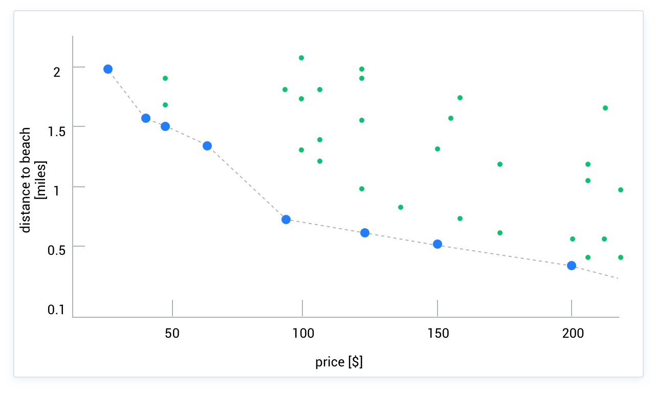
Given an object set O, the principle of skyline pruning is to find the set of objects that are not dominated by other objects. If object A is not dominated by object B in any dimension, and object A dominates object B in at least one dimension, object A dominates object B. In other words, the selection of dimensions and the definition of the domination relationship on each dimension are crucial. Suppose there are N index paths <idx_1, idx_2, idx_3...idx_n> available for the optimizer to choose from. For query Q, if index idx_x dominates index idx_y in the defined dimensions, index idx_y can be pruned in advance, preventing it from participating in the final cost computation.
Dimension definitions
For skyline pruning, the following three dimensions are defined for each index (the primary key is also considered an index):
Necessity for table read
Existence of an interesting order
Extraction of the query range from index prefixes
The following example is provided for analysis:
obclient> CREATE TABLE skyline(pk INT PRIMARY KEY,
    a INT,
    b INT,
    c INT,
    KEY idx_a_b(a, b),
    KEY idx_b_c(b, c),
    KEY idx_c_a(c, a)
    );
Table read: Indicates whether the query needs to read the primary table.
If the
idx_a_bindex is used, the primary table needs to be read because theccolumn is not present in theidx_a_bindex.obclient> SELECT /*+INDEX(skyline idx_a_b)*/ * FROM skyline;Interesting order: Determines whether a suitable order can be utilized.
The
idx_b_cindex can eliminate theORDER BYclause.obclient> SELECT pk, b FROM skyline ORDER BY b;Extraction of the query range from index prefixes.
Using the
idx_c_aindex allows quick location of the required row range without a full table scan.obclient> SELECT pk, b FROM skyline WHERE c > 100 AND c < 2000;
Based on these three dimensions, skyline pruning defines a domination relationship between indexes. If index A is not worse than index B in all three dimensions and is better than B in at least one dimension, it can be inferred that the final plan generated based on index B will not be better than that based on index A, so index B can be directly pruned. The judgment criteria are as follows:
If index
idx_Adoes not require a table read, but indexidx_Bdoes, indexidx_Adominatesidx_Bin this dimension.If the interesting order extracted from index
idx_Ais the vectorVa<a1, a2, a3 ...an>, and the interesting order extracted from indexidx_Bis the vectorVb<b1, b2, b3...bm>, andn > m, forai = bi (i=1..m), indexidx_Adominatesidx_Bin this dimension.If the set of columns that can be used to extract a query range from index
idx_AisSa<a1, a2, a3 ...an>, and the set for indexidx_BisSb <b1, b2, b3...bm>, andSais a superset ofSb, indexidx_Adominatesidx_Bin this dimension.
Table read
A table read checks whether the required columns are included in the index. Special considerations are needed for certain scenarios, such as when neither the primary table nor the index table has an interesting order and no query range can be extracted; in such cases, accessing the primary table directly may not be the optimal solution.
obclient> CREATE TABLE t1(pk INT PRIMARY KEY,
    a INT,
    b INT,
    c INT,
    v1 VARCHAR(1000),
    v2 VARCHAR(1000),
    v3 VARCHAR(1000),
    v4 VARCHAR(1000),
    INDEX idx_a_b(a, b)
    );
obclient>SELECT a, b,c FROM t1 WHERE b = 100;
Index |
Index Back |
Interesting Order |
Query Range |
|---|---|---|---|
| primary | no | no | no |
| idx_a_b | yes | no | no |
The index table is narrow compared with the primary table. Although the primary table dominates idx_a_b in the three dimensions, the cost of an index scan plus a table read is not necessarily higher than a full scan of the primary table. Simply put, the index table may only need to read one macroblock, while the primary table may need to read ten. In this case, the rule needs to be relaxed, and specific filter conditions must be considered comprehensively.
Interesting order
By utilizing the underlying order through an interesting order, the optimizer avoids sorting the rows scanned at the underlying layer, can eliminate ORDER BY, perform MERGE GROUP BY, and improve pipeline efficiency (without requiring materialization).
obclient> CREATE TABLE skyline(pk INT PRIMARY KEY,
    v1 INT,
    v2 INT,
    v3 INT,
    v4 INT,
    v5 INT,
    KEY idx_v1_v3_v5(v1, v3, v5),
    KEY idx_v3_v4(v3, v4)
    );
obclient> CREATE TABLE tmp (c1 INT PRIMARY KEY, c2 INT, c3 INT);
obclient> (SELECT DISTINCT v1, v3 FROM skyline JOIN tmp
    WHERE skyline.v1 = tmp.c1
    ORDER BY v1, v3)
    UNION (SELECT c1, c2 FROM tmp);
The execution plan shows that ORDER BY is eliminated, MERGE DISTINCT is applied, and sorting is also omitted for UNION. The order generated from the underlying TABLE SCAN can be used by upper-layer operators. In other words, retaining the row order from idx_v1_v3_v5 allows subsequent operators to perform better operations without changing the order. The optimizer can generate a better execution plan only when it recognizes these orders.
Therefore, when you perform skyline pruning based on the interesting order, you must take into consideration the order in which the indexes can make the maximum use. For example, the most useful order in the preceding example is (v1, v3) rather than just v1. The order (v1, v3) derived from the MERGE JOIN operator can also be used by the MERGE DISTINCT operator and then by the final UNION DISTINCT operator.
Query range
The extraction of the query range allows you to locate a specific macroblock at the underlying layer, reducing the I/O resource consumption at the storage layer.
For example, SELECT * FROM t1 WHERE pk < 100 AND pk > 0 can be applied to locate the specific macroblock by using the primary key index, making the query faster because a more accurate query range allows the database to scan fewer rows.
obclient> CREATE TABLE t1 (pk INT PRIMARY KEY,
    a INT,
    b INT,
    c INT,
    KEY idx_b_c(b, c),
    KEY idx_a_b(a, b)
    );
obclient> SELECT b FROM t1 WHERE a = 100 AND b > 2000;
For idx_b_c, the query range is (b), which can be extracted from its index prefix. For idx_a_b, the extracted query range is (a, b). So, idx_a_b dominates idx_b_c in this dimension.
Comprehensive example
obclient> CREATE TABLE skyline(pk INT PRIMARY KEY,
    v1 INT,
    v2 INT,
    v3 INT,
    v4 INT,
    v5 INT,
    KEY idx_v1_v3_v5(v1, v3, v5),
    KEY idx_v3_v4(v3, v4)
    );
obclient> CREATE TABLE tmp (c1 INT PRIMARY KEY, c2 INT, c3 INT);
obclient> SELECT MAX(v5) FROM skyline WHERE v1 = 100 AND v3 > 200 GROUP BY v1;
Index |
Index Back |
Interesting order |
Query range |
|---|---|---|---|
| primary | Not need | No | No |
| idx_v1_v3_v5 | Not need | (v1) | (v1, v3) |
| idx_v3_v4 | Need | No | (v3) |
It can be seen that index idx_v1_v3_v5 is not inferior to the primary key index or index idx_v3_v4 in any of the three dimensions. Therefore, according to Skyline pruning rules, the primary key index and index idx_v3_v4 are directly pruned. The proper definition of dimensions determines whether Skyline pruning is reasonable. Incorrect dimensions may cause an index to be pruned prematurely, potentially preventing the generation of an optimal plan.